LabxDB
LabxDB is versatile open-source solution for organizing and sharing structured data. LabxDB provides a toolkit to build browser-based graphical interface and REST interfaces to databases. Any table including nested tables in SQL server can be viewed/edited within a browser. Ready-to-use databases for laboratory (plasmid collection, high-throuput sequencing, ordering, etc) are already implemented.
Features
- Client-server architecture: multiple clients can access the database at the same time
- Support hierarchical data with unlimited number of nested levels
- Easy to add new databases using example databases provided
- Limited external dependencies for minimal long-term maintenance
- Open source license (MPL-2.0)
Technical implementation
- Back-end
- PostgreSQL database
- Written in Python using asynchronous I/O aiohttp
- Front-end
- Written in plain Javascript ES6 without external dependencies.
Implemented databases
Databases are implemented using LabxDB for biology lab (see architecture for detailed description):
- LabxDB seq: High-throughput sequencing data
- Lab collections: plasmid, cell lines, fish or fly lines
- Lab management: Order (purchase)
Printable manual
This documentation is available as a printable manual.
License
LabxDB is licensed under the terms of the Mozilla Public License 2.0.
Architecture
The back-end runs on the server. It stores data in SQL server and prepares the data to be sent to the front-end. The front-end runs within the user’s browser.
Back-end
The back-end provides REST API distributing the data and the meta-information associated with the data to the client. The data are stored in PostgreSQL tables. The meta-information comprises how the data are structured, their type (integer, date etc), how to display them to users and how users can input/edit them. The structure of the data is composed of nested level(s). Each level is stored in separate table in the database.
The back-end handles different types of requests. Some user requests are sending an output to the front-end (GET) while others are only requiring some input (POST). All requests are handled by handlers. LabxDB provides 5 different types of handlers characterized by their input(s) and output(s). For each type of handler corresponds one Python class. When implementing a specific request in a database, the class that implements this request is inheriting from one of these generic classes. The 5 generic classes of handlers are (source code in handlers/generic.py):
| Class | HTTP request | GET returns | Usage |
|---|---|---|---|
GenericHandler |
GET and POST | HTML page | Main handler providing the data to the client (GET request). The search_criterion, sort_criterion and limit parameters submitted with POST request are used to search, sort or limit the data respectively. |
GenericQueriesHandler |
GET and POST | HTML page | Handler used to create new data. Compatible with creating single or multiples records. GET request provides meta-information while the POST request handles adding the data to the database. |
GenericRecordHandler |
GET and POST | HTML page | Similar handler to GenericQueriesHandler but for a single record. The record_id is mandatory for both GET and POST requests. |
GenericGetHandler |
GET | JSON | Simple handler to get a record identified by its record_id. |
GenericRemoveHandler |
GET | JSON | Simple handler to remove a record identified by its record_id. |
The back-end is written in Python with queries written in SQL and PL/pgSQL.
Front-end
For displaying the data, LabxDB defines the Board class (source code in board.js). This class is inherited by two classes: the Table and TreeBlock classes. The Table class displays within a table a single level of a database. To display multiple levels, the TreeBlock class has been implemented. The Toolbar class (source code in toolbar.js) can be used with a Board to allow users to filter, sort etc data.
To edit the data, LabxDB defines the Form class (source code in form.js). If users are required to input manually each field, the TableForm class is appropriate. It can be used to edit a single or multiple records. In case users can provide input as, for example, tabulated text, the BatchForm class is recommended.
The back-end is written in plain ES6 Javascript with no external dependencies.
Communications between back-end and front-end
Data are sent as JSON data by the back-end to the front-end. Most data are produced as JSON directly by the PostgreSQL server.
The meta-information is defined in the back-end. It is transmitted to the client as Javascript code. Transformation is done using the Jinja2 template engine. To one front-end class and one back-end class corresponds a template. For example, the template defined in generic_tree.jinja is designed to be used with front-end TreeBlock and the back-end GenericHandler. Templates include code to instantiate these classes on the client.
Extending features of generic classes
On the back-end, classes written for specific database inherit the generic handlers. By design each handler inherits from a single generic handlers.
On the front-end, classes such as TreeBlock can be used directly. If some of the methods of these classes needs to be overloaded, developer can write a new class inheriting or not from theses provided classes. The class to be used is defined in the back-end. The template in the back-end includes automatically the necessary code to load the file defining the class and the code to instantiate it in the client browser.
Implemented databases
Several databases are implemented using LabxDB. Intended use is for scientific laboratory. The most complex is LabxDB seq database which includes multiple levels and GUI views extending the default LabxDB views. Multiple laboratory collections such as plasmids or oligos are implemented. The LabxDB order database is the most simple with a single table and using only generic handlers.
LabxDB seq
LabxDB seq is designed to store genomic high-throughput sequencing sample annotations. It’s composed of 4 tables: project, sample, replicate and run. It is the most complex database developed with LabxDB. The management of genomic sequencing data is implemented from manual annotation of samples (sample label etc) to automatic attribution of IDs to samples. Data are organized in projects containing samples, themselves containing replicates, which are divided into runs. Runs represent the level annotating the raw sequencing data (often FASTQ files).
LabxDB mutant
LabxDB mutant is composed of two tables: gene and allele. The allele table is a sub-level of the gene table. In a biology laboratory, this database helps to track mutants generated targeting genes and the characteristics of each specific allele of the genes. For each gene, multiple alleles can be characterized for a gene. The same architecture could be used to track fly or cell lines. This database can be used to start developing a database with more than one level.
LabxDB plasmid
LabxDB order is composed of a single table storing a collection of plasmids. Plasmid ID are automatically attributed and users can attached a screenshot of the plasmid map to each plasmid record.
LabxDB order
LabxDB order is composed of a single table developed to track ordering in lab. This is the most simple database developed with LabxDB and as such the most appropriate to start implementing a new database with LabxDB.
LabxDB oligo
LabxDB oligo is composed of a single table developed to track oligo sequences in lab. Using PL/pgSQL (SQL Procedural Language), database attributes automatically an ID to each oligo (i.e item in the database). This insure oligo are always receiving a unique ID. This ID is used to physically label the tube containing the oligo, track and store it.
LabxDB seq
Schema
LabxDB seq is composed of 3 levels: project, sample, replicate and run. Each level is stored in a table. Columns within each table are described here.

Tools
With provided scripts sequencing data and their annotations can be imported and exported from sequencing center and external resources such as SRA.
| Script | Function |
|---|---|
| import_seq | Import your sequencing data from your local sequencing center. |
| export_sra | Export your sequencing data annotations to SRA. Prepare tabulated files for SRA import with your annotations. |
| export_sra_fastq | Export your sequencing data to SRA. Prepare FASTQ file(s). Helper script of export_sra. |
| import_sra_id | Import SRA IDs to your sequencing data annotations, i.e. import SRRxxx, SRPxxx etc to your database. |
| import_sra | Import SRA data (FASTQ and annotations). |

Installation
These steps have to be done only the first time data is downloaded and imported.
-
Install LabxDB Python module including scripts.
-
Create folders
Choose a root folder for your sequencing data, here this will be
/data/seq. Then create the following sub-folders:mkdir /data mkdir /data/seq mkdir /data/seq/raw # For RAW sequencing data mkdir /data/seq/by_run # For symbolic links to sequencing runs mkdir /data/seq/prepared # For imported/reformated sequencing data
Tutorials
| Tutorial | Script | Description |
|---|---|---|
| Tutorial 1 | import_seq |
How to import your high-throughput sequencing data in LabxDB seq? From downloading data from your sequencing center to annotate samples. |
| Tutorial 2 | export_sra |
How to export your high-throughput sequencing data to SRA? This greatly simplify export your own data to SRA at the time of publication. |
| Tutorial 3 | import_sra |
How to import publicly available high-throughput sequencing data from SRA? |
| Tutorial 4 | import_sra_id |
How to import the SRA attributed by SRA to your high-throughput sequencing data after import to SRA? Importing SRA IDs to your database allows you to keep track of exported (i.e. published) or not samples. |
LabxDB seq tables
Project table
| Column | Description |
|---|---|
| Project ref | Project reference (ID), i.e. AGPxxx (Two initials + P) |
| Project name | Project name. A computer-oriented name: short, no space. Used by post-processing pipelines folder names etc. |
| Short label | As short as possible label (to fit small spaces such as genome track label). Use abbreviations. Populated while creating the annotation structure. |
| Long label | More descriptive label. Longer than short label. No abbreviation. Include all conditions, genotypes, timepoints and treatments. |
| Scientist | Scientist initials. |
| External scientist | In case this project is imported (from SRA for example) or in collaboration, enter that scientist name. |
| SRA ref | SRPxxx ID (for project imported from SRA). |
Sample table
| Column | Type | Description |
|---|---|---|
| Sample ref | Sample reference (ID), i.e. AGSxxx (Two initials + S) | |
| Project ref | Project reference (ID). Structure column: which project this sample belongs to. | |
| Short label | Short label using abbreviation. Include genotype, timepoint and condition. | |
| Long label | Long label without abbreviation. Expands short label. | |
| Species | fish | Species (danRer, homSap, droMel etc). |
| Maternal strain | fish | Genotype of mother if not wild-type. |
| Paternal strain | fish | Genotype of father if not wild-type. |
| Genotype | fish | “WT” or specific genotype. |
| Ploidy | fish | “2n” if diploid or “n” if haploid. |
| Age (hpf) | fish | Age in hours post-fertilization. |
| Stage | fish | Developmental stage embryos were collected. |
| Tissue | fish | If specific tissue was collected. |
| Condition | library | If experiment is done in pair (or more) such as CLIP/input, CLIP/IgG or RPF/input, enter the condition. |
| Treatment | library | Chemical treatment applied such as morpholino, cycloheximide. |
| Selection | library | Selection or purification of library such as poly(A) (abbreviated “pA”), ribo-zero (abbreviated “r0”) or antibodies. |
| Molecule | library | Sequenced molecule: “mRNA” for mRNA-seq, “RNA” for CLIP or “DNA” for ChIP-seq. |
| Library protocol | library | Protocol used to prepared the library such as dUTP or sRNA (small RNA). |
| Adapter 5' | library | Name of 5’ adapter. |
| Adapter 3' | library | Name of 3’ adapter. |
| Track priority | Genome track priority. Track with lowest number comes first. | |
| Track color | Genome track color name. | |
| SRA ref | SISxxx ID (for SRA Imported Sample). | |
| Notes | Any information not input in other columns. |
Replicate table
| Column | Description |
|---|---|
| Replicate ref | Replicate reference (ID), i.e. AGNxxx (Two initials + N) |
| Replicate order | Number. First, second or third (etc) replicates. |
| Sample ref | Sample reference (ID). Structure column: which sample this replicate belongs to. |
| Short label | Short label using abbreviation. Include genotype, timepoint and condition. Include replicate number (for example with B1, B2). |
| Long label | Long label without abbreviation. Expands short label. Include replicate number. |
| SRA ref | SINxxx ID (for SRA Imported Replicate). |
| Publication ref | If replicate has been published, name of publication. |
| Notes | Any information not input in other columns. |
Run table
| Column | Description |
|---|---|
| Run ref | Run reference (ID), i.e. AGRxxx (Two initials + R) |
| Run order | Number. First, second or third (etc) runs. |
| Replicate ref | Replicate reference (ID). Structure column: which replicate this run belongs to. |
| Tube label | Label used on tube sent to sequencing facility. Filename of FASTQ files. |
| Barcode | Illumina barcode if samples were multiplexed. |
| Second barcode | Internal barcode if samples were multiplexed using a second barcode. |
| Request | Internal reference for sequencing request. |
| Request date | Date of internal sequencing request. |
| Failed | Did this sequencing run failed? |
| Flowcell | Flowcell reference. |
| Platform | Name of platform used for sequencing. For example “Illumina NovaSeq 6000”. |
| Quality scores | Quality scores coding within FASTQ files. Most recent scores are coded with “Illumina 1.8”. |
| Directional | Is read direction (5’ to 3’ for example) preserved during library preparation? |
| Paired | Single-end or paired-end sequencing. |
| Read1 strand | If read is directional, what is the orientation of read 1. Example: mRNA-seq prepared with dUTP is “-” or antisense. CLIP or small-RNA-seq are “+” or sense. Most DNA sequencing is “u” unstranded. Important for read mapping. |
| Spots | Number of spots. |
| Max read length | Length of longest read in run. |
| SRA ref | SRRxxx ID (for run imported from SRA). |
| Notes | Any information not input in other columns. |
Tutorial: Import your data
How to import high-throughput sequencing data in LabxDB seq using import_seq? Tutorial is divided in 3 parts:
- Download the sequencing data
- Annotate the project(s), sample(s), replicate(s) and run(s) that compose your data.
- Post-processing the sequencing data.
Imported data were published in Vejnar et al.
Importing sequencing data
Download
The import_seq script encapsulates all operations required to manage the high-throughput sequencing data. It will:
- Download the data from a remote location such as a sequencing center,
- Format the data to comply with a common format. This includes by default renaming files and compressing the FASTQ files with a more efficient algorithm than Gzip.
- Input the sequencing run(s) into the database.
The data (FASTQ files) are downloaded into the folder /data/seq/raw/LABXDB_EXP in the following example. By default, import_seq will download data in folder with current date.
Imported data were published in Vejnar et al. For this tutorial, only a few reads were kept per runs to reduce the file sizes.
import_seq --bulk 'LABXDB_EXP' \
           --url_remote 'https://labxdb.vejnar.org/doc/databases/seq/import_seq/example/' \
           --ref_prefix 'TMP_' \
           --path_seq_raw '/data/seq/raw' \
           --squashfs_download \
           --processor '4' \
           --make_download \
           --make_format \
           --make_staging
The sequencing runs will receive temporary IDs prefixed with TMP_. To import multiple projects, different prefixes such TMP_User1 or TMP_User2 can be used.
If you didn’t install Squashfs, you can:
- Remove
--squashfs_downloadoption and no archive.sqfs will be created and download directory will remain or, - Replace
--squashfs_downloadwith--delete_downloadoption to delete the non-FASTQ files.
After import
After completion, sequencing data can be found in /data/seq/raw:
/data/seq/raw
└── [ 172]  LABXDB_EXP
    ├── [4.0K]  archive.sqfs
    ├── [ 254]  resa-2h-1_R1.fastq.zst
    ├── [ 271]  resa-6h-1_R1.fastq.zst
    ├── [ 254]  resa-6h-2a_R1.fastq.zst
    └── [ 348]  resa-6h-2b_R1.fastq.zst
- FASTQ files were compressed with Zstandard.
- Remaining files (all but FASTQ files) were archived with Squashfs.
In the Run view of LabxDB seq, the 4 runs were imported:
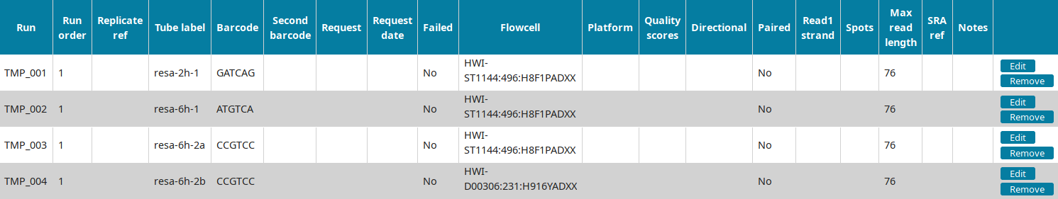
You can then proceed to Annotating sequencing data.
Annotating sequencing data
Creating the annotation structure
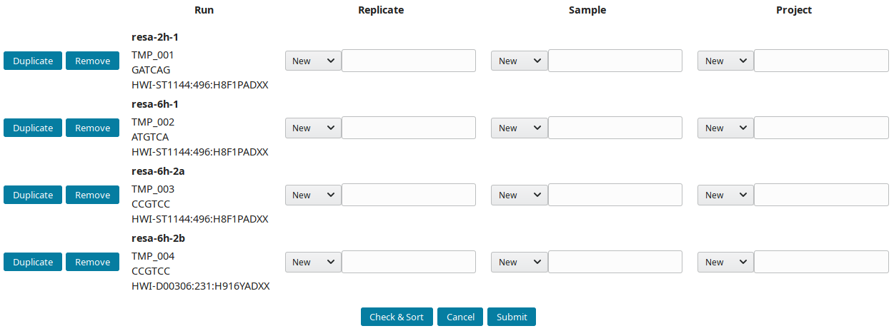
After downloading and importing the sequencing runs, they can be grouped into replicate(s), sample(s) and project(s). The New runs view was implemented to create this tree-like structure:
-
By default, all new runs are displayed in the New runs view. To select a subset of runs, search for a pattern in the top toolbar. For example, to select runs with
TMP_User1prefix use:
These prefixes were assigned using the
--ref_prefixofimport_seq. -
References (IDs) are prefixed by default with AG (AGP, AGS, AGN and AGR for project, sample, replicate and run respectively). Input preferred prefix in the input field:

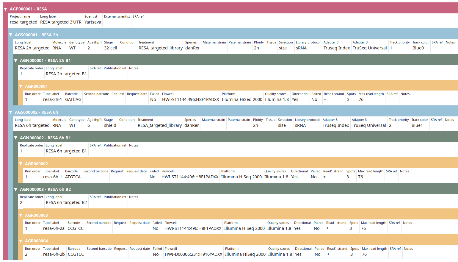
The structure of the example runs is (B1 and B2 are the first and second biological replicates):
Project  Sample  Replicate  Run (temporary ID)
RESA ___ 2h ___  2h B1 ____ resa-2h-1  (TMP_001)
     \__ 6h ___  6h B1 ____ resa-6h-1  (TMP_002)
            \__  6h B2 ____ resa-6h-2a (TMP_003)
                       \___ resa-6h-2b (TMP_004)
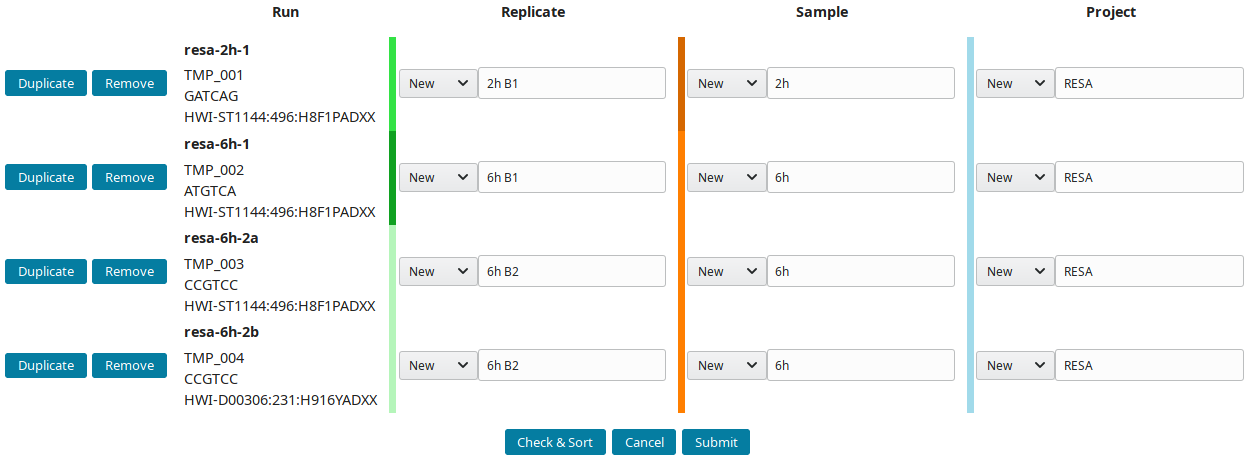
The project RESA was composed of 2 samples (experiments performed at 2 time-points, 2 and 6 hours). The first sample 2h was done in one replicate (B1) while 6h sample was replicated twice (B1 and B2). Replicates were sequenced one, except 6h B2, which was sequenced twice. Using this information, the labels can be input. These labels are entered as Short labels in the database. To validate your input, click on Check & Sort. This will sort the samples and highlight the structure of your annotation:
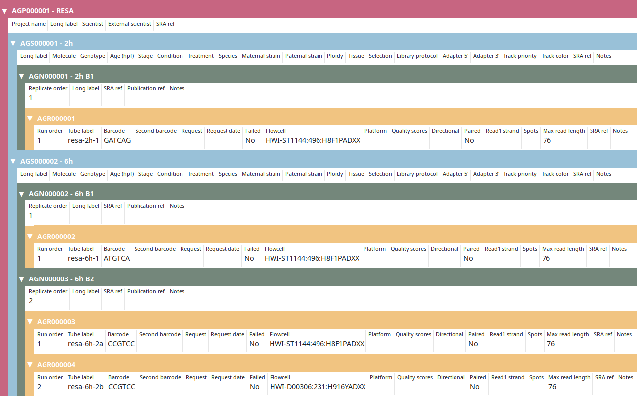
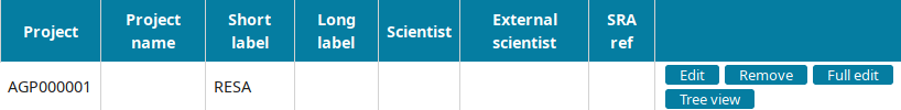
Then submit to let LabxDB seq create the new replicates, samples and project. Use the Tree view to display the new project:
Project annotation
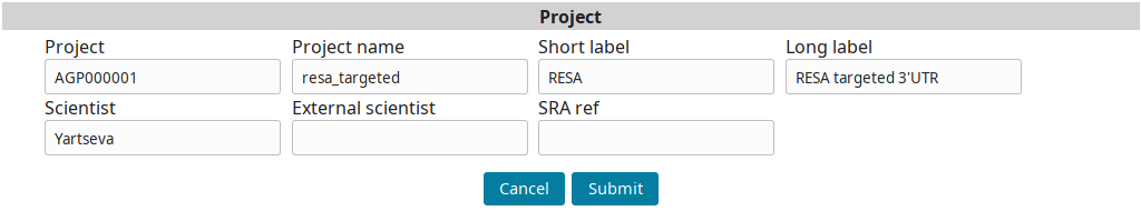
Go to the Project view to find the newly created project and click on Edit.
Input the project information and submit you input:
Sample annotation
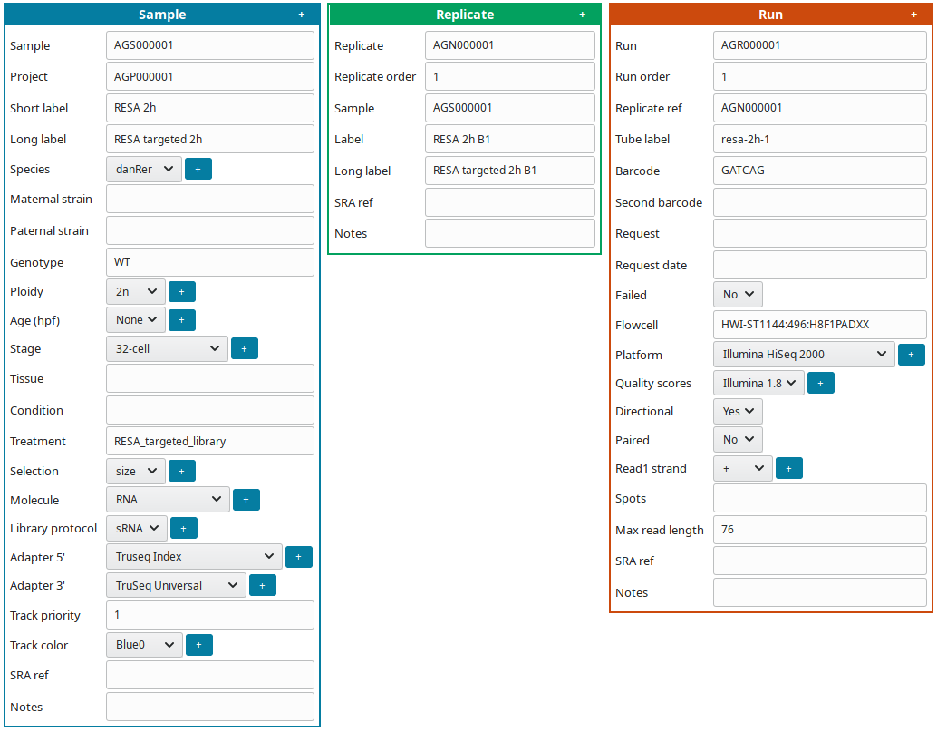
To edit at the same time all sample(s), replicate(s) and run(s), click on Full edit on the Project view. In this view, each sample and descendant replicate(s) and run(s) are presented together in a block:
To facilitate editing annotations:
-
Use helping tools:
- Click on the
+symbol (1) to displayCopybutton. - Click on a
Copybutton (2) to replicate the same information on all cells of the same type.
For example, if all samples are from the same species, input the species, click
+(1), them copy the species on all samples (2):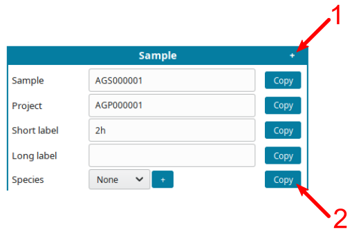
- Click on the
-
Save your annotations in the database by pressing
Submitbutton regularly to avoid loosing any input. -
For dropdown fields: if your entry is missing, click on
+button to add a new category.
Once done click on the Submit & exit button. Back on the Project view, display the finished annotation using the Tree view button:
You can then proceed to Post-processing data.
Post-processing data
To simplify downstream analysis of sequencing data, import_seq can create links to FASTQ files for each sequencing run. Finding all FASTQ files for a specific run is then trivial and doesn’t require any information beyong the run reference. Run import_seq with:
import_seq --bulk 'LABXDB_EXP' \
           --path_seq_raw '/data/seq/raw' \
           --path_seq_run '/data/seq/by_run' \
           --make_import
Output will display the imported runs:
Summary
resa-2h-1                     HWI-ST1144:496:H8F1PADXX      GATCAG                        AGR000001      /data/seq/raw/H8F1PADXX
resa-6h-1                     HWI-ST1144:496:H8F1PADXX      ATGTCA                        AGR000002      /data/seq/raw/H8F1PADXX
resa-6h-2a                    HWI-ST1144:496:H8F1PADXX      CCGTCC                        AGR000003      /data/seq/raw/H8F1PADXX
resa-6h-2b                    HWI-D00306:231:H916YADXX      CCGTCC                        AGR000004      /data/seq/raw/H8F1PADXX
And the following links will be created:
by_run/
├── AGR000001
│   └── resa-2h-1_R1.fastq.zst -> ../../raw/H8F1PADXX/resa-2h-1_R1.fastq.zst
├── AGR000002
│   └── resa-6h-1_R1.fastq.zst -> ../../raw/H8F1PADXX/resa-6h-1_R1.fastq.zst
├── AGR000003
│   └── resa-6h-2a_R1.fastq.zst -> ../../raw/H8F1PADXX/resa-6h-2a_R1.fastq.zst
└── AGR000004
    └── resa-6h-2b_R1.fastq.zst -> ../../raw/H8F1PADXX/resa-6h-2b_R1.fastq.zst
Tutorial: Export your data to SRA
The export_sra script prepares your sample annotations to easily export them into SRA. It export annotations into tabulated files following SRA expected format. The associated script export_sra_fastq prepared the FASTQ files, ready to be uploaded into SRA. This process is required when publishing your data.
Requirement
For this tutorial, it is expected that the tutorial to import your own data has been followed. To skip this tutorial and start at the same stage,
-
Empty the seq tables. Execute
psql -U postgresto connect to PostgreSQL server and execute:TRUNCATE seq.project; TRUNCATE seq.sample; TRUNCATE seq.replicate; TRUNCATE seq.run;Exit PostgreSQL.
-
Import the annotations (SQL files are available here):
psql -U postgres < seq_project.sql
psql -U postgres < seq_sample.sql
psql -U postgres < seq_replicate.sql
psql -U postgres < seq_run.sql
Export annotations
To export the three replicates from the RESA project, execute:
export_sra --replicates AGN000001,AGN000002,AGN000003
The labels used internally in your database might be different than the appropriates labels for SRA. To apply filters on labels, add the --path_label_filters option. Filters are submitted in a CSV file: the first column is the string to be replaced by the string defined in the second column. For example:
RESA,RESA (RNA-element selection assay)
To use the filter (saved in filters.csv), execute:
export_sra --replicates AGN000001,AGN000002,AGN000003 \
           --path_label_filters filters.csv
export_sra will create:
sra_samples.tsvwith the sample annotationssra_data.tsvwith a list of exported FASTQ filessra_exported.tsvwith already SRA exported samples files
How to use these files is explained in the next section.
Export FASTQ files
To prepare the corresponding FASTQ files using the data.json created in the previous step, execute:
export_sra_fastq --path_seq_raw '/data/seq/raw' \
                 --path_seq_run '/data/seq/by_run' \
                 --path_data data.json
The following files will be created:
├── AGR000001_R1.fastq.gz
├── AGR000002_R1.fastq.gz
├── AGR000003_R1.fastq.gz
├── AGR000004_R1.fastq.gz
├── data.json
├── sra_data.tsv
├── sra_exported.tsv
└── sra_samples.tsv
Submit to SRA
To submit samples to SRA, login to the Submission Portal and go to the Sequence Read Archive (SRA).
Then click on the New submission button to start a new submission:

Fill the different forms. Use the sra_samples.tsv and sra_data.tsv files in the appropriate tabs.
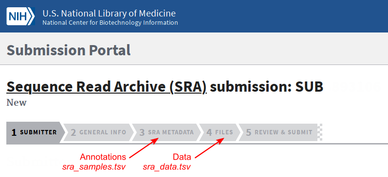
At the end of the submission, you can upload the FASTQ files.
Tutorial: Import data from SRA
The import_sra script imports data and sample annotations from publicly available publicly available high-throughput sequencing data from SRA. It will:
- Downloads the FASTQ files,
- Format the data to comply with a common format. This includes by default renaming files, compressing the FASTQ files with a more efficient algorithm than Gzip, and stripping read names.
- Input the sequencing run(s) into the database.
Download
Imported data were published in Yartseva et al under accession SRP090954.
import_sra --project SRP090954 \
           --runs SRR4375304,SRR4375305 \
           --path_seq_run /data/seq/by_run \
           --path_seq_prepared /data/seq/prepared \
           --dump_sra \
           --db_import \
           --create_links
The --dump_sra option downloads and gets FASTQ files, --db_import imports samples and runs into the database, while --create_links creates the symbolic links to /data/seq/by_run.
--project option is used, all runs will be imported. If only a few runs are needed, use the --runs option.
This command returns:
Downloading infos # 0 ID 3268484
Downloading infos # 1 ID 3268483
Downloading infos # 2 ID 3268482
Downloading infos # 3 ID 3268481
Downloading infos # 4 ID 3268480
Downloading infos # 5 ID 3268479
Downloading infos # 6 ID 3268478
Downloading infos # 7 ID 3268477
Downloading infos # 8 ID 3268463
Downloading infos # 9 ID 3268411
Downloading infos # 10 ID 3268394
Downloading infos # 11 ID 3268393
Downloading infos # 12 ID 3268378
Downloading infos # 13 ID 3268358
Downloading infos # 14 ID 3268357
Downloading infos # 15 ID 3268356
Downloading infos # 16 ID 3268355
Downloading infos # 17 ID 3268354
Downloading infos # 18 ID 3268353
Downloading infos # 19 ID 3268352
Downloading infos # 20 ID 3268351
Downloading infos # 21 ID 3268350
Downloading infos # 22 ID 3268349

RESA identifies mRNA regulatory sequences with high resolution
SRS1732690          RESA-Seq - WT 8h pA r3 B1
   \_SRR4375304
SRS1732691          RESA-Seq - WT 8h pA r3 B2
   \_SRR4375305

Import to DB
Dump from SRA
Download and dump SRR4375304
join   :|-------------------------------------------------- 100.00%
concat :|-------------------------------------------------- 100.00%
spots read      : 5,896,053
reads read      : 11,792,106
reads written   : 11,792,106
SRR4375304_R1.fastq  : 20.71%   (1036594224 => 214688034 bytes, SRR4375304_R1.fastq.zst)
SRR4375304_R2.fastq  : 20.44%   (1036594224 => 211867665 bytes, SRR4375304_R2.fastq.zst)
Download and dump SRR4375305
join   :|-------------------------------------------------- 100.00%
concat :|-------------------------------------------------- 100.00%
spots read      : 8,845,249
reads read      : 17,690,498
reads written   : 17,690,498
SRR4375305_R1.fastq  : 20.35%   (1555652720 => 316532334 bytes, SRR4375305_R1.fastq.zst)
SRR4375305_R2.fastq  : 20.83%   (1555652720 => 324036832 bytes, SRR4375305_R2.fastq.zst)
Imported runs from the SRP090954 project are large. For a quick test of import_sra, import SRR1761155 from SRP052298.
import_sra --project SRP052298 \
           --runs SRR1761155 \
           --path_seq_run /data/seq/by_run \
           --path_seq_prepared /data/seq/prepared \
           --dump_sra \
           --db_import \
           --create_links
Result
Files
The import_sra script creates the following files including the data files (in prepared folder as files are converted from SRA to FASTQ files) and symbolic links:
/data/seq
├── [4.0K]  by_run
│   ├── [4.0K]  SRR4375304
│   │   ├── [  48]  SRR4375304_R1.fastq.zst -> ../../prepared/SRP090954/SRR4375304_R1.fastq.zst
│   │   └── [  48]  SRR4375304_R2.fastq.zst -> ../../prepared/SRP090954/SRR4375304_R2.fastq.zst
│   └── [4.0K]  SRR4375305
│       ├── [  48]  SRR4375305_R1.fastq.zst -> ../../prepared/SRP090954/SRR4375305_R1.fastq.zst
│       └── [  48]  SRR4375305_R2.fastq.zst -> ../../prepared/SRP090954/SRR4375305_R2.fastq.zst
└── [4.0K]  prepared
    └── [4.0K]  SRP090954
        ├── [205M]  SRR4375304_R1.fastq.zst
        ├── [202M]  SRR4375304_R2.fastq.zst
        ├── [302M]  SRR4375305_R1.fastq.zst
        └── [309M]  SRR4375305_R2.fastq.zst
Annotations
The import_sra script imports the sequencing run(s) into the database. Use the Tree view to display the new project:
- SRPxxx and SRRxxx IDs are conserved and imported as-is from SRA.
- SISxxx (SRA Import Sample) and (SRA Import N replicate) are created as no IDs in SRA correspond to LabxDB definition of samples and replicates and not all data providers interpret the definition of SRA samples the same way.
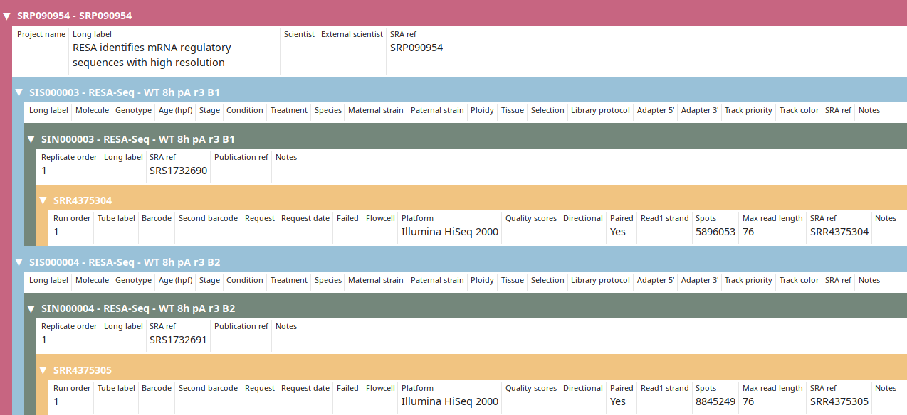
After annotations are imported from SRA, project and sample can be further annotated manually.
Tutorial: Import IDs from SRA
After exporting your high-throughput sequencing data to SRA, SRA will attribute IDs to them. This tutorial explains how to use the script import_sra_id to import these SRA IDs and link them to your internal IDs. This allows you to keep track of published data within your own database.
To perform this linkage, import_sra_id uses two pieces of information:
- the number of spots (i.e. reads) sequenced,
- the columns
sample_refandreplicate_refadded as supplementary annotations during SRA export byexport_srascript. For example, see SRP189389 to find an example containing these columns.
Requirement
For this tutorial, it is expected that some data have been already exported to SRA. When you imported annotations following the Import your data tutorial, IDs were automatically attributed. But we attributed different IDs in our database. For the importing of SRA IDs to work, the local and SRA IDs need to be the same. To import our annotations:
-
Empty the seq tables. Execute
psql -U postgresto connect to PostgreSQL server and execute:TRUNCATE seq.project; TRUNCATE seq.sample; TRUNCATE seq.replicate; TRUNCATE seq.run;Exit Postgresql.
-
Import the annotations (SQL files are available here):
psql -U postgres < seq_project.sql
psql -U postgres < seq_sample.sql
psql -U postgres < seq_replicate.sql
psql -U postgres < seq_run.sql
You can then check that you imported the data properly:
Observe that the IDs and the number of spots have been updated to new ones (compared to tutorial).
Create publication
Go to the Publications tab and click on the Add new Publication button to go the new publication form.
Use the following data:
| Column | Description |
|---|---|
| Publication (short internal name for publication) | vejnar_messih_genome_research_2019 |
| Title | Genome wide analysis of 3’-UTR sequence elements and proteins regulating mRNA stability during maternal-to-zygotic transition in zebrafish |
| Publication date | 2019-07-01 |
| Pubmed ID | 31227602 |
| SRA ref (comma separated list of SRP IDs) | SRP189512,SRP189389,SRP189499 |
…to fill the form:
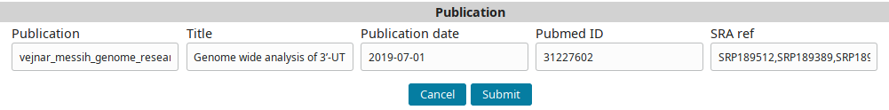
And submit to add the publication record.
Import
SRA IDs can then be imported using the --update option.
import_sra_id --update \
              --publication_ref vejnar_messih_genome_research_2019 \
              --dry | grep -v WARNING
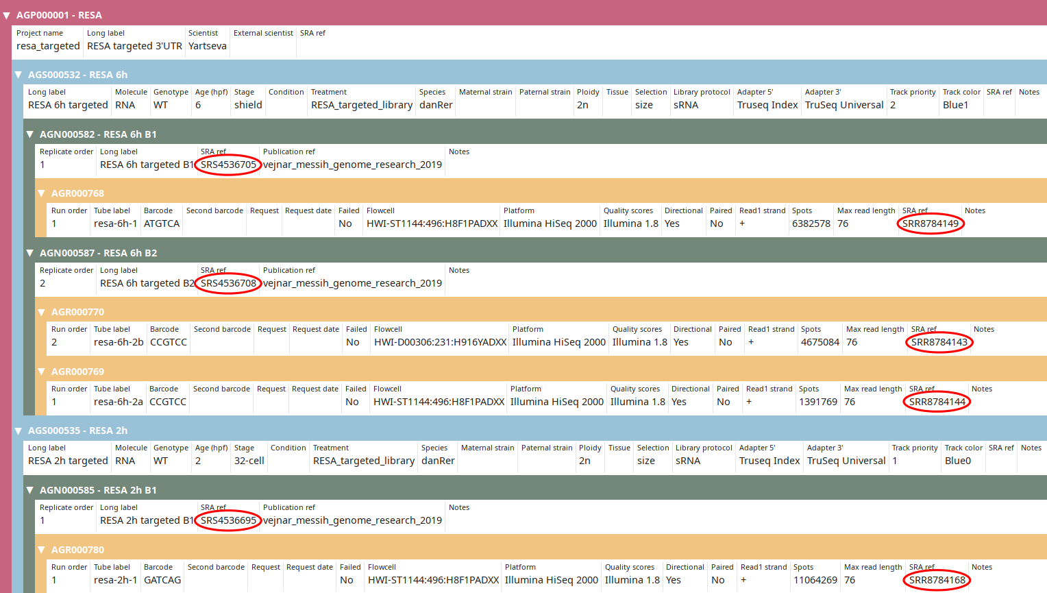
import_sra_id won’t be able to find all the runs published within these SRA projects. It will display a warning for each unfound run. We suggest to first filter the numerous warnings. Run the command again the command without the | grep -v WARNING pipe to display these warnings.
This command returns:
Title: Genome wide analysis of 3’-UTR sequence elements and proteins regulating mRNA stability during maternal-to-zygotic transition in zebrafish
Loading SRP189512

> SRP189512
Loading SRP189389

> SRP189389
  Replicate
  > Local: AGN000585  RESA 2h B1
  > SRA:   RESA - WT 32c r2 B1 AGN000585             SRS4536695
    > Run: SRR8784168
  Replicate
  > Local: AGN000582  RESA 6h B1
  > SRA:   RESA - WT 6h r2 B1 AGN000582              SRS4536705
    > Run: SRR8784149
  Replicate
  > Local: AGN000587  RESA 6h B2
  > SRA:   RESA - WT 6h r2 B2 AGN000587              SRS4536708
    > Run: SRR8784143
  Replicate
  > Local: AGN000587  RESA 6h B2
  > SRA:   RESA - WT 6h r2 B2 AGN000587              SRS4536708
    > Run: SRR8784144
Loading SRP189499

> SRP189499

...
Once you got this output, execute the command again without the --dry option:
import_sra_id --update \
              --publication_ref vejnar_messih_genome_research_2019 | grep -v WARNING
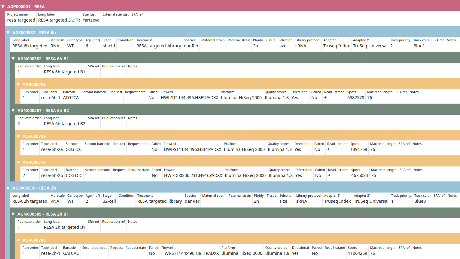
Now the SRA IDs should be imported as you can see in the tree view:
Installation
Installation instructions are available for:
-
Server: To install LabxDB on a server.
-
Python Client: To use Python code to interact with LabxDB.
Server installation
Requirements
-
PostgreSQL server
-
Python 3.6+
-
Python libraries aiohttp, aiohttp-jinja2 and asyncpg.
pip3 install aiohttp
pip3 install aiohttp-jinja2
pip3 install asyncpg
Installing a database
labxdb_install.sh available in the contrib/virt folder of LabxDB repository installs LabxDB and its dependencies. Please refer to this script for details about LabxDB installation.
-
Install PostgreSQL server, Python and Python libraries.
-
Create a
labrole to connect to PostgreSQL. -
Import schema describing a database. Example databases are available in
contrib/databases/sqlfolder of the LabxDB repository. The schema are templates. To load them and replace the variables in the templates, the simple scripttpl_sql.pycan be used. To connect to PostgreSQL server, a user with admin rights, here postgres, is required.tpl_sql.py -s -a schema,purchase -u postgres create_order_tables.sql -
Start LabxDB server application. For example:
app.py --port=8081 --db_host=localhost --db_user=lab --db_password="labxdb" --db_name=postgres --db_conn=2
Python client
Installation
-
LabxDB-tools depends on requests, urllib3 and pyfnutils Python modules. To install it and its dependencies:
pip3 install labxdb-tools --user -
Make sure
$HOME/.local/binis in your PATH; the scriptimport_seqfor example should be executable. If not, configure your PATH in your~/.bashrc:export PATH=$PATH:$HOME/.local/bin
Dependencies
-
import_seq
Install zstd, wget and squashfs-tools with your favourite package manager. For example:
pacman -S zstd wget squashfs-toolsNotesquashfs-toolsis not mandatory. After download, remaining files can be (i) kept as-is or (ii) deleted using the option--delete_download. -
import_sra
Install
fastq-dumpfrom the NCBI SRA (Sequence Read Archive) tools:wget https://ftp-trace.ncbi.nlm.nih.gov/sra/sdk/current/sratoolkit.current-ubuntu64.tar.gz tar xvfz sratoolkit.current-ubuntu64.tar.gz cp sratoolkit.*-ubuntu64/bin/fastq-dump-orig* $HOME/.local/bin/fastq-dump
Configuration
To access LabxDB databases, clients need URL, path, login and passwords. They can be provided as environment variables or in a configuration file.
By environment variables
In your '~/.bashrc:
export LABXDB_HTTP_URL="http://127.0.0.1:8081/"
export LABXDB_HTTP_PATH_SEQ="seq/"
export LABXDB_HTTP_LOGIN=""
export LABXDB_HTTP_PASSWORD=""
By configuration file
In any file within any of these folders:
$HTS_CONFIG_PATH.HTS_CONFIG_PATHcan be defined by the user.$XDG_CONFIG_HOME/hts.XDG_CONFIG_HOMEis defined by your desktop environment.
Example configuration:
- Create a folder
/etc/hts - Open a file
/etc/hts/labxdb.jsonand write (in JSON format):{ "labxdb_http_url": "http://127.0.0.1:8081/", "labxdb_http_path_seq": "seq/", "labxdb_http_login": "", "labxdb_http_password": "" } - Open a file
/etc/hts/path.jsonand write (in JSON format):{ "path_seq_raw": "/data/seq/raw", "path_seq_run": "/data/seq/by_run", "path_seq_prepared": "/data/seq/prepared" } - Add in
~/.bashrc:export HTS_CONFIG_PATH="/etc/hts"
--path_config option. All scripts in LabxDB-python accept this option.
Deploy LabxDB
Deploy a ready-to-use LabxDB. Provided scripts can create OS images or install LabxDB in the cloud.
- Images for Virtualbox or QEMU are provided. For lightweight solution, Docker configuration file is provided. Easy, free and quick way to test or deploy LabxDB.
- Using the same scripts, LabxDB can be installed in the cloud, for example using DigitalOcean or Vultr. Easy, not free, way to test or deploy LabxDB. Installed instance in the cloud will be publicly accessible on internet.
The installation is split into two parts:
- LabxDB installation. LabxDB is ready to use and accessible on the port 8081 with an URL like
http://IP:8081. To be used for testing or within an existing web server. - Public-facing LabxDB installation. On top of the previous install, it adds:
- A reverse-proxy, Caddy, exposing LabxDB on secure https using a domain name provided by DuckDNS (or any registrar, for example Gandi) and SSL certificates signed by Let’s Encrypt.
- A firewall Nftables. By default only port 22 (SSH), 80 and 443 (web) are open.
Options
-
Technologies
Lightweight virtualization Virtualization Cloud Docker VirtualBox DigitalOcean QEMU Vultr -
Type of installations (by script)
Type Script LabxDB installation labxdb_install.shPublic-facing LabxDB installation dns_nft_caddy.sh
Deploy with QEMU
A pre-installed LabxDB image for QEMU is available to easily run LabxDB. It provides a fully functional LabxDB based on the ArchLinux operating system.
Start virtual machine
To get the LabxDB virtual machine running:
- Install QEMU
- Download the LabxDB virtual machine labxdb.qcow2.zst
- Unzip the virtual machine using Zstandard:
zstd -d labxdb.qcow2.zst - Start LabxDB virtual machine. For example:
qemu-system-x86_64 -machine q35,accel=kvm \
                   -cpu host \
                   -enable-kvm \
                   -m 2000 \
                   -smp 1 \
                   -drive file=labxdb.qcow2,if=virtio,cache=writeback,discard=ignore,format=qcow2 \
                   -device virtio-net,netdev=n1 \
                   -netdev user,id=n1,hostfwd=tcp::8022-:22,hostfwd=tcp::8081-:8081
Connect to LabxDB
The LabxDB client should be available at http://localhost:8081.
Configure the virtual machine
To admin the virtual, SSH server is running on the virtual machine. To connect using SSH client:
ssh -p 8022 root@127.0.0.1
The pre-configured root password is archadmin.
arch_install.sh to install ArchLinux and ii) the script labxdb_install.sh to install LabxDB and its dependencies. These scripts are available in the contrib/virt folder of LabxDB repository. Please refer to these scripts for details about the virtual machine setup.
Deploy with VirtualBox
A pre-installed LabxDB image for Oracle VM VirtualBox is available to easily run LabxDB. It provides a fully functional LabxDB based on the ArchLinux operating system.
Start virtual machine
To get the LabxDB virtual machine running:
- Install VirtualBox
- Download the LabxDB virtual machine labxdb.ova
- Import LabxDB virtual machine as explained in VirtualBox manual
- Start LabxDB virtual machine
Connect to LabxDB
The LabxDB web interface should be available at http://localhost:8081.
Configure the virtual machine
To admin the virtual, SSH server is running on the virtual machine. To connect using SSH client:
ssh -p 8022 root@127.0.0.1
The pre-configured root password is archadmin.
arch_install.sh to install ArchLinux and ii) the script labxdb_install.sh to install LabxDB and its dependencies. These scripts are available in the contrib/virt folder of LabxDB repository. Please refer to these scripts for details about the virtual machine setup.
Deploy with Docker
Docker provides a lightweight virtualization to use LabxDB. A Dockerfile can be used to build a LabxDB image automatically based on Debian GNU/Linux operating system.
Install Docker and start the docker service.
Build the debian/labxdb image
docker build -f Dockerfile -t debian/labxdb .
You can then see the newly built image using the following command:
docker images
Start the debian/labxdb image
To start debian/labxdb image, use the following command:
docker run -it -p 8081:8081 debian/labxdb
The web interface runs on port 8081 which is exposed on the Docker interface also on port 8081.
Deploy to DigitalOcean
This tutorial explains how to deploy LabxDB in the cloud using DigitalOcean. For a few dollars per month, you can run LabxDB following the easy setup explained here.
Login to DigitalOcean
- Create a login at DigitalOcean
- Login to your account DigitalOcean login page.
Add SSH key
To connect to your server, a droplet in DigitalOcean vernacular, your SSH login key will be installed by the installation script.
Generate your SSH key
If you don’t already have an SSH key, follow this guide to generate one.
Load your SSH key
After logging in, go to the Security tab of the Account section. Click on Add SSH key:
And copy-paste your SSH key and give it a name:
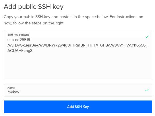
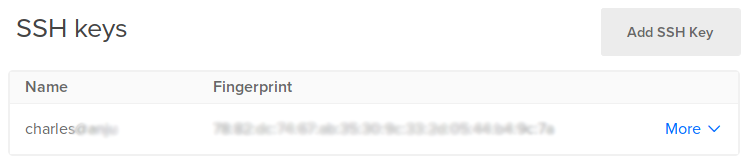
You can then see you added SSH key:
This process is further explained in this tutorial.
Create droplet
Configure droplet
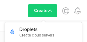
Go to Create Droplets by clicking on the Create button and select Droplets:
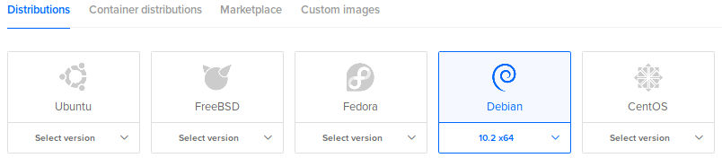
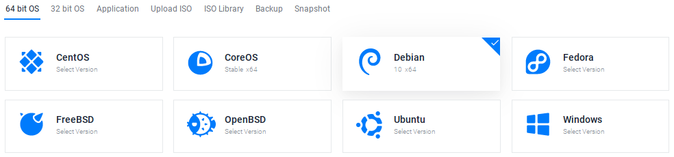
Choose an image and version (Debian 10):
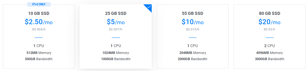
Choose a plan:
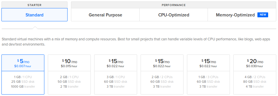
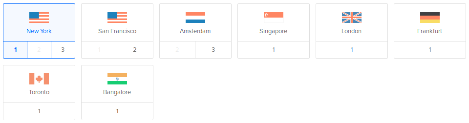
Choose a region:
In Select additional options, select User data:
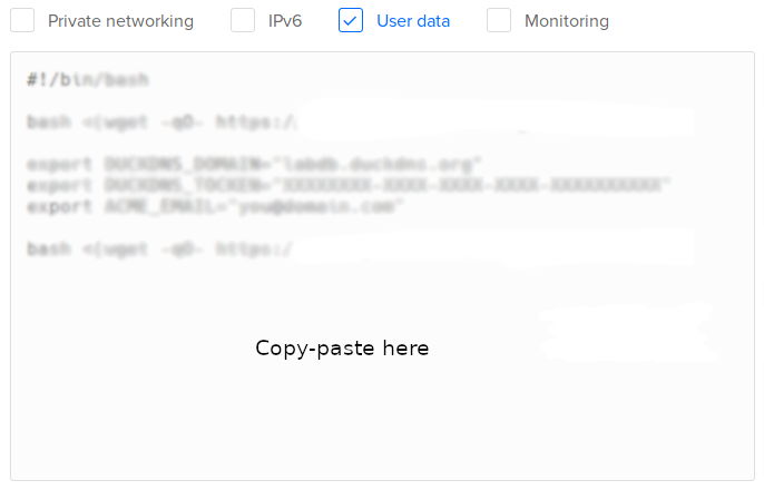
Copy-paste one of the following scripts:
- Test version. Installs LabxDB:
#!/bin/bash bash <(wget -qO- https://git.sr.ht/~vejnar/LabxDB/blob/main/contrib/virt/labxdb_install.sh) - Production version. Installs LabxDB with domain name and security (https+firewall):
NoteWith the parameter
ACME_STAGING="yes", the Let’s Encrypt Staging Environment will be used to sign the SSL certificate. The resulting certificate won’t be usable in internet browsers. This is intented to test deploying LabxDB. To use the regular Let’s Encrypt server, change the parameter toACME_STAGING="no"as described in the post-installation section.- If you created a DuckDNS domain, set DUCKDNS_DOMAIN, DUCKDNS_TOCKEN and ACME_EMAIL (with your email) variables (see here)
#!/bin/bash bash <(wget -qO- https://git.sr.ht/~vejnar/LabxDB/blob/main/contrib/virt/labxdb_install.sh) export DUCKDNS_DOMAIN="labxdb.duckdns.org" export DUCKDNS_TOCKEN="XXXXXXXX-XXXX-XXXX-XXXX-XXXXXXXXXX" export ACME_EMAIL="you@domain.com" export ACME_STAGING="yes" bash <(wget -qO- https://git.sr.ht/~vejnar/LabxDB/blob/main/contrib/virt/dns_nft_caddy.sh) - If you have your own domain name, set DOMAIN (with your domain) and ACME_EMAIL (with your email) variables:
NoteThe installation does not set the IP of your new droplet to your domain name. As a consequence, the certificate creation will fail. Once the droplet installation, restart Caddy as described in the post-installation section to create a valid certificate.
#!/bin/bash

bash <(wget -qO- https://git.sr.ht/~vejnar/LabxDB/blob/main/contrib/virt/labxdb_install.sh)

export DOMAIN="labxdb.mydomain.com"
export ACME_EMAIL="you@domain.com"
export ACME_STAGING="yes"

bash <(wget -qO- https://git.sr.ht/~vejnar/LabxDB/blob/main/contrib/virt/dns_nft_caddy.sh)
- If you created a DuckDNS domain, set DUCKDNS_DOMAIN, DUCKDNS_TOCKEN and ACME_EMAIL (with your email) variables (see here)
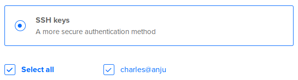
In Authentication, select SSH keys:
Choose a hostname:
Then Create your new droplet.
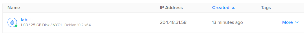
Start droplet
Go back to main panel at Droplets and wait for the new droplet to be ready:
Post-installation
If you used your own domain name or created a staging domain name using ACME_STAGING="yes", follow these steps to create a valid certificate (be aware of limits):
- Only if you used your own domain name to install a production version: set the IP (in our example
204.48.31.58) of your new droplet to your domain name (at your domain name registrar or DNS provider). Wait a few minutes for the update to be applied. - Only if you are ready to create a production certificate, login to your instance, open with an editor
/etc/caddy/caddy.jsonand update the ACME server from the staging to the production URL by replacing:by:{ "module": "acme", "ca": "https://acme-staging-v02.api.letsencrypt.org/directory" }{ "module": "acme", "ca": "https://acme-v02.api.letsencrypt.org/directory" } - Login to your instance and restart Caddy using (it forces creating a new certificate):
systemctl restart caddy
Connect to LabxDB
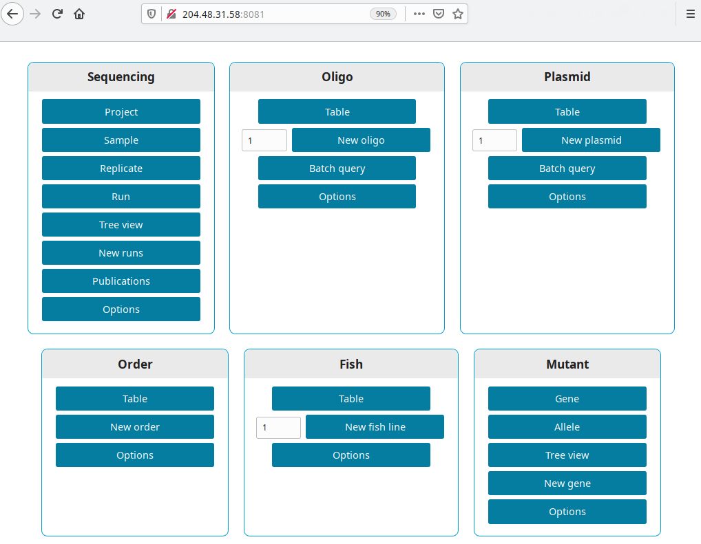
Test version
Get the IP from your new droplet (in our example 204.48.31.58). Open a browser and go to http://your ip:8081, i.e. http://204.48.31.58:8081.
Production version
LabxDB is accessible at the domain you set in DUCKDNS_DOMAIN or DOMAIN. For our example https://labxdb.duckdns.org.
The password is defined in /etc/caddy/caddy.json within the http_basic module. To define a new password, it needs to be encoded using:
caddy hash-password
More help is available here.
More configuration
Connect to droplet
Connect with SSH to your droplet using:
ssh root@204.48.31.58
Or, if you setup a domain name (labxdb.duckdns.org here):
ssh root@labxdb.duckdns.org
Troubleshooting
In case the installation is incomplete or failed, the log of install script is saved in /var/log/cloud-init-output.log.
DigitalOcean documentation
DigitalOcean documentation is available for further help.
Deploy to Vultr
This tutorial explains how to deploy LabxDB in the cloud using Vultr. For a few dollars per month, you can run LabxDB following the easy setup explained here.
Login to Vultr
Add SSH key
To connect to your server, an instance in DigitalOcean vernacular, your SSH login key will be installed by the installation script.
Generate your SSH key
If you don’t already have an SSH key, follow this guide to generate one.
Load your SSH key
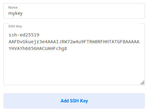
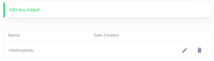
After logging in, go to the SSH Keys tab of the Products section. Click on Add SSH Key, and copy-paste your SSH key and give it a name:
You can then see you added SSH key:
This process is further explained in this tutorial.
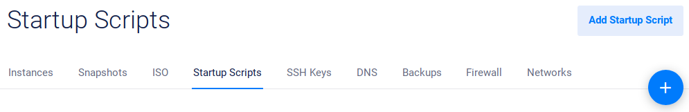
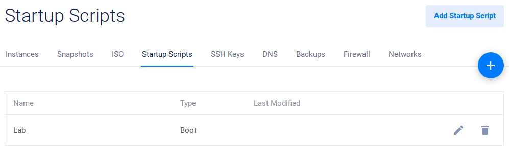
Add Startup Script
After logging in, go to Startup Scripts. After Vultr install a functional Linux distribution on your virtual server, this script will be used to install LabxDB automatically.
Click on the Add Startup Script button:
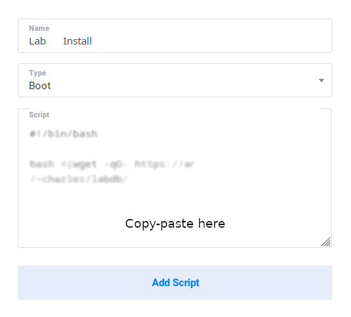
Input the LabxDB script in the form with the following parameters:
-
Name: LabxDB
-
Type: Boot
-
Script: Copy-paste one of the following scripts:
- Test version. Installs LabxDB:
#!/bin/bash bash <(wget -qO- https://git.sr.ht/~vejnar/LabxDB/blob/main/contrib/virt/labxdb_install.sh) - Production version. Installs LabxDB with domain name and security (https+firewall):
NoteWith the parameter
ACME_STAGING="yes", the Let’s Encrypt Staging Environment will be used to sign the SSL certificate. The resulting certificate won’t be usable in internet browsers. This is intented to test deploying LabxDB. To use the regular Let’s Encrypt server, change the parameter toACME_STAGING="no"as described in the post-installation section.- If you created a DuckDNS domain, set DUCKDNS_DOMAIN, DUCKDNS_TOCKEN and ACME_EMAIL (with your email) variables (see here)
#!/bin/bash bash <(wget -qO- https://git.sr.ht/~vejnar/LabxDB/blob/main/contrib/virt/labxdb_install.sh) export DUCKDNS_DOMAIN="labxdb.duckdns.org" export DUCKDNS_TOCKEN="XXXXXXXX-XXXX-XXXX-XXXX-XXXXXXXXXX" export ACME_EMAIL="you@domain.com" export ACME_STAGING="yes" bash <(wget -qO- https://git.sr.ht/~vejnar/LabxDB/blob/main/contrib/virt/dns_nft_caddy.sh) - If you have your own domain name, set DOMAIN (with your domain) and ACME_EMAIL (with your email) variables:
NoteThe installation does not set the IP of your new instance to your domain name. In consequence, the certificate creation will fail. Once the instance installation, restart Caddy as described in the post-installation section.
#!/bin/bash

bash <(wget -qO- https://git.sr.ht/~vejnar/LabxDB/blob/main/contrib/virt/labxdb_install.sh)

export DOMAIN="labxdb.mydomain.com"
export ACME_EMAIL="you@domain.com"
export ACME_STAGING="yes"

bash <(wget -qO- https://git.sr.ht/~vejnar/LabxDB/blob/main/contrib/virt/dns_nft_caddy.sh)
- If you created a DuckDNS domain, set DUCKDNS_DOMAIN, DUCKDNS_TOCKEN and ACME_EMAIL (with your email) variables (see here)
- Test version. Installs LabxDB:
Then click Add Script:
The new script should then be available:
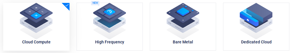
Create instance
Configure instance
Go to Deploy New Instance by clicking on the Plus button (Deploy New Server):
Choose a node type:
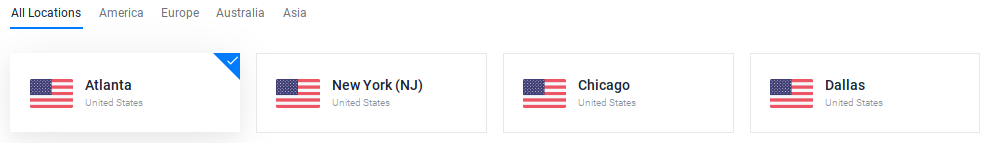
Choose a region:
Choose the Debian image (and latest version):
Choose a node size:
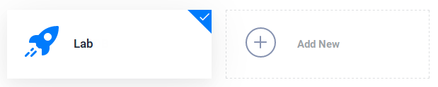
Select the Startup Script you entered at the previous step:
Select an SSH key if you configured one.
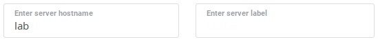
Choose a Server Hostname and Label:
Then Deploy your new instance.
Start instance
Go back to main panel at https://my.vultr.com and wait for the new instance to be ready:
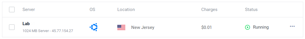
Post-installation
If you used your own domain name or created a staging domain name using ACME_STAGING="yes", follow these steps to create a valid certificate (be aware of limits):
- Only if you used your own domain name to install a production version: set the IP (in our example
45.77.154.27) of your new instance to your domain name (at your domain name registrar or DNS provider). Wait a few minutes for the update to be applied. - Only if you are ready to create a production certificate, login to your instance, open with an editor
/etc/caddy/caddy.jsonand update the ACME server from the staging to the production URL by replacing:by:{ "module": "acme", "ca": "https://acme-staging-v02.api.letsencrypt.org/directory" }{ "module": "acme", "ca": "https://acme-v02.api.letsencrypt.org/directory" } - Login to your instance and restart Caddy using (it forces creating a new certificate):
systemctl restart caddy
Connect to LabxDB
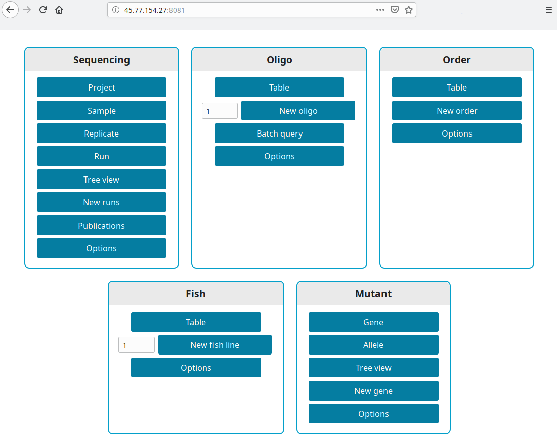
Test version
Get the IP from your new instance (in our example 45.77.154.27). Open a browser and go to http://your ip:8081, i.e. http://45.77.154.27:8081.
Production version
LabxDB is accessible at the domain you set in DUCKDNS_DOMAIN or DOMAIN. For our example https://labxdb.duckdns.org.
The password is defined in /etc/caddy/caddy.json within the http_basic module. To define a new password, it needs to be encoded using:
caddy hash-password
More help is available here.
More configuration
Connect to instance
Click on the new instance to get Server information. On this page, you can find the root password.
Connect with SSH to your instance using:
ssh root@45.77.154.27
Or, if you setup a domain name (labxdb.duckdns.org here):
ssh root@labxdb.duckdns.org
Troubleshooting
In case the installation is incomplete or failed, the log of install script is saved in /tmp/firstboot.log.
Vultr documentation
Vultr documentation is available for further help.
Helpers
Generate your SSH key
In a Terminal on your computer, run:
ssh-keygen -t ed25519
This command will generate the following output:
Generating public/private ed25519 key pair.
Enter file in which to save the key (/Users/***/.ssh/id_ed25519):
Enter passphrase (empty for no passphrase):
Enter same passphrase again:
Your identification has been saved in /Users/***/.ssh/id_ed25519.
Your public key has been saved in /Users/***/.ssh/id_ed25519.pub.
- Press Enter to confirm the default name of the file containing the key
- Don’t enter any passphrase: press Enter twice
Finally the key is generated and a randomart image is displayed.
The key fingerprint is:
SHA256:***

The key's randomart image is:
+--[ED25519 256]--+
|  ..++.o         |
| .   .-          |
|.  . .           |
| .=  ..          |
|.  oo ..n.       |
| .. o+.oo        |
|.. . *=..+ ..    |
|..E+. +=B =o..   |
|o.o o+==oB=+o.   |
+----[SHA256]-----+
Display your public key with:
cat ~/.ssh/id_ed25519.pub
This command will generate the following output (with your own key):
ssh-ed25519 AAFDvGkuejr3e4AAAIJRW72w4u9FTRmBRFHHTATGFBAAAAAYHVAYh6656HACUAHFchg8 charles@server
Domain name
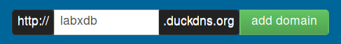
For public-facing LabxDB installation, a domain name is required. With DuckDNS, you can get a domain like something.duckdns.org, with something of your choice. It’s free and supported by donations.
-
To create a subdomain, login with Twitter, Github, Reddit or Google login.
-
Once logged in, create a subdomain of your choice. Here labxdb:
-
To modify the IP associated with your domain, keep in a safe place your token:

Creating a new LabxDB database
This tutorial uses the example of the Order database to detail the design of a new database in LabxDB.
The Order database aims to help tracking ordering (purchases) in a laboratory. Multiple members of the laboratory can enter new items to purchase while members (same members or not) order them. Since in most labs, members who need new items don’t often have the authorization to order, the database keeps track of which items are needed and the current state of orders. It also tracks spending over time.
The files created during this tutorial are:
| Purpose | Path |
|---|---|
| SQL schemas | contrib/databases/sql/create_order_tables.sql |
| Back-end | handlers/order.py |
| Front-end | static/js/order/board.js |
| Front-end | static/js/order/addon.js |
Creating the tables in PostgreSQL
Each database is stored in a different schema. For this database, the purchase schema will be used.
CREATE SCHEMA purchase;
The main table for this database contains the items to be bought. The item_id column is required in each LabxDB table to identify uniquely each record. Other columns do not have any restriction.
CREATE TABLE purchase.item (
    item_id serial not null,
    item varchar(255),
    item_ref varchar(255),
    item_size varchar(255),
    provider varchar(255),
    provider_stockroom boolean,
    quantity integer,
    unit_price numeric(8,2),
    total_price numeric(8,2),
    status varchar(50),
    recipient varchar(50),
    date_insert date default CURRENT_DATE,
    date_order date,
    manufacturer varchar(255),
    manufacturer_ref varchar(255),
    funding varchar(255),
    PRIMARY KEY (item_id));
Some columns are stored as text but only a limited number of options are available to users (with a drop-down menu; see below). To store these options, a dedicated option table is required. All 3 columns are required.
CREATE TABLE purchase.option (
    option_id serial not null,
    group_name varchar(50) not null,
    option varchar(50) not null,
    UNIQUE (group_name, option),
    PRIMARY KEY (option_id));
Finally, permissions to edit the database are given to the lab user used by the back-end.
GRANT USAGE ON SCHEMA purchase TO lab;
GRANT SELECT,INSERT,UPDATE,DELETE ON TABLE purchase.item TO lab;
GRANT SELECT,UPDATE ON TABLE purchase.item_item_id_seq TO lab;
GRANT SELECT,INSERT,UPDATE,DELETE ON TABLE purchase.option TO lab;
GRANT SELECT,UPDATE ON TABLE purchase.option_option_id_seq TO lab;
Back-end
BaseHandler
The back-end defines a BaseHandler class containing the database meta-information in common between all handlers. All handlers inherit this class.
The class variables defined in the BaseHandler are:
| Variable | Description |
|---|---|
| name | The main name of the database |
| schema | The name of the schema in PostgreSQL storing the data |
| levels | Level(s) used by the handler (identified by order in level_infos) |
| level_infos | Description of each level with label, url and column_id (serial ID) fields |
| column_infos | Description of columns (see table below) |
| column_titles | List of columns used as title in the tree view |
| default_search_criterions | Default search criterions applied after client page load |
| default_sort_criterions | Default sort criterions applied after client page load |
| default_limits | Default limits applied after client page load |
| columns | List of displayed columns |
| form | Definition of edit form (see below) |
| board_class | The front-end board class to use for board view |
| form_class | The front-end form class to use for form view |
Applied to the Order database, OrderBaseHandler inherits from BaseHandler:
class OrderBaseHandler(base.BaseHandler):
    name = 'order'        # The main name of the database
    schema = 'purchase'   # The name of the schema in PostgreSQL storing the data

    levels = [0]                       # This database has a single level `item`.
    levels_json = json.dumps(levels)   # Metainformation as JSON. Used in the template to communicate to the client.

    level_infos = [{'label': 'Order', 'url': 'order', 'column_id': 'item_id'}] # Each level `label`, `url` and `column_id`.
    level_infos_json = json.dumps(level_infos)

    column_infos = [{'item_id': {'search_type': 'equal_number', 'gui_type': 'text', 'required': True, 'label': 'Order ID', 'tooltip': ''},
                     'item': {'search_type': 'ilike', 'gui_type': 'text', 'required': True, 'label': 'Item', 'tooltip': ''},
                     'item_ref': {'search_type': 'ilike', 'gui_type': 'text', 'required': False, 'label': 'Item ref', 'tooltip': 'Item reference or Catalog number'},
                     'item_size': {'search_type': 'ilike', 'gui_type': 'text', 'required': False, 'label': 'Size', 'tooltip': ''},
                     'provider': {'search_type': 'ilike', 'gui_type': 'select_option_none', 'required': False, 'label': 'Provider', 'tooltip': 'Where to order?'},
                     'provider_stockroom': {'search_type': 'equal_bool', 'gui_type': 'select_bool_none', 'required': True, 'label': 'Skr', 'tooltip': 'Is this item available in the stockroom?'},
                     'quantity': {'search_type': 'equal_number', 'gui_type': 'text', 'required': False, 'label': 'Qty', 'tooltip': ''},
                     'unit_price': {'search_type': 'equal_number', 'gui_type': 'text', 'required': False, 'label': 'Price', 'tooltip': 'Price per unit'},
                     'total_price': {'search_type': 'equal_number', 'gui_type': 'text', 'required': False, 'label': 'Total', 'tooltip': '', 'button': {'label': 'Update total', 'click': 'order_total'}},
                     'status': {'search_type': 'ilike', 'gui_type': 'select_option_none', 'required': True, 'label': 'Status', 'tooltip': '', 'default':'init_status'},
                     'recipient': {'search_type': 'ilike', 'gui_type': 'select_option_none', 'required': True, 'label': 'Recipient', 'tooltip': ''},
                     'date_insert': {'search_type': 'equal_date', 'gui_type': 'text', 'required': True, 'pattern': '[0-9][0-9][0-9][0-9]-[0-9][0-9]-[0-9][0-9]', 'label': 'Date', 'tooltip': 'Order creation date', 'button': {'label': 'Today', 'click': 'order_today'}, 'default':'init_date'},
                     'date_order': {'search_type': 'equal_date', 'gui_type': 'text', 'required': False, 'pattern': '[0-9][0-9][0-9][0-9]-[0-9][0-9]-[0-9][0-9]', 'label': 'Order', 'tooltip': '', 'button': {'label': 'Today', 'click': 'order_today_status'}},
                     'manufacturer': {'search_type': 'ilike', 'gui_type': 'text', 'required': False, 'label': 'Manufacturer', 'tooltip': ''},
                     'manufacturer_ref': {'search_type': 'ilike', 'gui_type': 'text', 'required': False, 'label': 'Manufacturer ref', 'tooltip': ''},
                     'funding': {'search_type': 'ilike', 'gui_type': 'text', 'required': False, 'label': 'Funding', 'tooltip': ''}}]
    column_infos_json = json.dumps(column_infos)

    column_titles = []
    column_titles_json = json.dumps(column_titles)

    default_search_criterions = [];
    default_search_criterions_json = json.dumps(default_search_criterions)

    default_sort_criterions = []
    default_sort_criterions_json = json.dumps(default_sort_criterions)

    default_limits = [['All', 'ALL', False], ['10', '10', False], ['100', '100', True], ['500', '500', False]]
    default_limits_json = json.dumps(default_limits)

    columns = []
    columns_json = json.dumps(columns)

    form = []
    form_json = json.dumps(form)

    board_class = 'Table'          # The default front-end board class to use for board view
    form_class = 'TableForm'       # The default front-end form class to use for form view
The meta-information about columns is defined in the column_infos class variable using the keys:
| Key | Definition |
|---|---|
| search_type | ilike or equal_number (ILIKE or = SQL operators to search within this column) |
| gui_type | text, select_option_none (drop-down menu with options) or select_bool_none (drop-down menu with yes/no/None options) |
| required | HTML5 required: True or False |
| label | text |
| tooltip | text |
| pattern | HTML5 pattern to restrict user input. |
| onload | Define the function to start when edit field is loaded. |
| button | Define the button to add next to edit field. Button defined by label and onclick. |
The meta-information about forms is defined in the form class variable, containing a list of sections to include in the form.
| Key | Definition |
|---|---|
| label | Label of form section. None if no label |
| columns | List of columns to edit in this section |
DefaultHandler
The DefaultHandler defined the default view of the database in default_url. It inherits from GenericDefaultHandler and OrderBaseHandler.
@routes.view('/order')
class OrderDefaultHandler(generic.GenericDefaultHandler, OrderBaseHandler):
    default_url = 'order/table'
GenericHandler
OrderHandler handles the main table of the Order database. Defaults defined in the OrderBaseHandler are adapted to this view. The specific class variables are:
| Variable | Definition |
|---|---|
| queries | List of template SQL queries for each level of the database. Each level has a search_query_level and sort_query_level. |
| queries_search_prefixes | List of prefix for each level. Only defined as WHERE for first level and AND for subsequent level(s) in existing databases. |
@routes.view('/order/table')
class OrderHandler(generic.GenericHandler, OrderBaseHandler):
    tpl = 'generic_table.jinja'
    board_class = 'OrderTable'

    levels = [0]
    levels_json = json.dumps(levels)

    default_sort_criterions = [[0, 'date_order', 'DESC', 'Order'], [0, 'provider_stockroom', 'ASC', 'Skr'], [0, 'provider', 'ASC', 'Provider']]
    default_sort_criterions_json = json.dumps(default_sort_criterions)

    columns = [[{'name':'item'}, {'name':'item_ref'}, {'name':'item_size'}, {'name':'provider'}, {'name':'provider_stockroom'}, {'name':'unit_price'}, {'name':'quantity'}, {'name':'total_price'}, {'name':'status'}, {'name':'recipient'}, {'name':'date_insert'}, {'name':'date_order'}, {'name':'manufacturer'}, {'name':'manufacturer_ref'}, {'name':'funding'}]]
    columns_json = json.dumps(columns)

    queries = ["SELECT COALESCE(array_to_json(array_agg(row_to_json(r))), '[]') FROM (SELECT * FROM %s.item {search_query_level0} {sort_query_level0} LIMIT {limit}) r;"%OrderBaseHandler.schema]
    queries_search_prefixes = [[' WHERE ']]
GenericQueriesHandler
The GenericQueriesHandler is designed to handle new data input. Multiple records can be input at the same time. Class variables includes the form (see above) and insert_queries. The template queries must include columns and query_values variables that will contain the list of columns included in the form and list of values edited by the user respectively.
@routes.view('/order/new')
class OrderNewHandler(generic.GenericQueriesHandler, OrderBaseHandler):
    tpl = 'generic_edit.jinja'

    form = [{'label':'Order', 'columns':[{'name':'item'}, {'name':'item_ref'}, {'name':'item_size'}, {'name':'date_insert'}, {'name':'recipient'}, {'name':'funding'}]},
            {'label':None, 'columns':[{'name':'unit_price'}, {'name':'quantity'}, {'name':'total_price'}]},
            {'label':'Status', 'columns':[{'name':'status'}, {'name':'date_order'}]},
            {'label':'Provider', 'columns':[{'name':'provider'}, {'name':'provider_stockroom'}, {'name':'manufacturer'}, {'name':'manufacturer_ref'}]}]
    form_json = json.dumps(form)

    insert_queries = ["INSERT INTO %s.item ({columns}) VALUES ({query_values});"%OrderBaseHandler.schema]
GenericRecordHandler
The GenericRecordHandler is designed to handle data editing of a single record. Class variables includes the form (see above) and update_queries. This handler reuses the form from OrderNewHandler. The template queries must include update_query and record_id variables.
@routes.view('/order/edit/{record_id}')
class OrderEditHandler(generic.GenericRecordHandler, OrderBaseHandler):
    tpl = 'generic_edit.jinja'
    form_class = 'TableForm'

    form = OrderNewHandler.form
    form_json = OrderNewHandler.form_json

    update_queries = ["UPDATE %s.item SET {update_query} WHERE item_id={record_id};"%OrderBaseHandler.schema]
GenericGetHandler
The GenericRecordHandler is designed to handle getting a single record. The template queries must include record_id variable.
@routes.view('/order/get/{record_id}')
class OrderGetHandler(generic.GenericGetHandler, OrderBaseHandler):
    queries = ["SELECT COALESCE(array_to_json(array_agg(row_to_json(r))), '[]') FROM (SELECT * FROM %s.item WHERE item_id={record_id}) r;"%OrderBaseHandler.schema]
GenericRemoveHandler
The GenericRecordHandler is designed to handle removal of a single record. The template queries must include record_id variable.
@routes.view('/order/remove/{record_id}')
class OrderRemoveHandler(generic.GenericRemoveHandler, OrderBaseHandler):
    queries = ["DELETE FROM %s.item WHERE item_id={record_id};"%OrderBaseHandler.schema]
Front-end
The main view handled by OrderHandler uses the Table class. To allow users to easily duplicate an order (to reorder the same item again), a new button has been added. The getControlElements method is overloaded to add this button in OrderTable (set in board_class), which inherits from the Table class. This new class is defined in order_board.js. The code to load this file in the client is automatically added by generic_table.jinja template.
class OrderTable extends Table {
    getControlElements(record) {
        var cts = []
        // Edit, Remove, and Duplicate
        cts.push(this.getControlEdit(record))
        cts.push(this.getControlRemove(record))
        cts.push(this.getControlDuplicate(record))
        // Ordered
        var button = createElement("BUTTON", "button", "Ordered")
        button.type = "submit"
        button.action = this.getActionURL("edit", record)
        button.onclick = function (e) {
            var xhr = new XMLHttpRequest()
            // Post
            xhr.open("POST", e.target.action, true)
            xhr.responseType = "text"
            xhr.onload = function() {
                if (this.status == 200) {
                    var status = this.getResponseHeader("Query-Status")
                    if (status == "OK") {
                        window.location.reload()
                    } else {
                        alert("Query failed: " + status)
                    }
                } else {
                    alert("Request failed: " + this.statusText)
                }
            }
            // Prepare
            var data = [{"status": "ordered", "date_order": getDate()}]
            // Send
            xhr.send(JSON.stringify(data))
        }
        cts.push(button)
        // Return
        return cts
    }
}
In OrderBaseHandler, click and default actions are defined for controls in the editing form. They are coded in order/addon.js. The code to load this file in the client is automatically added by generic_edit.jinja template.
function addonStart(op, t, e) {
    let r
    switch (op) {
        case 'init_date':
            r = initDate(t)
            break
        case 'init_status':
            r = initStatus(t)
            break
        case 'order_today_status':
            r = orderTodayStatus(t)
            break
        case 'order_today':
            r = orderToday(t)
            break
        case 'order_total':
            r = orderTotal(t)
            break
        default:
            alert('Unknown operation: '+op)
    }
    return r
}

function initDate(input) {
    return getDate()
}

function initStatus(input) {
    return 'to order'
}
Finally, add a new entry in the main.jinja template.
Updates
Version 0.4.0
This version replaces the procedure (written in PL/pgSQL) assigning automatically IDs in LabxDB seq by the equivalent Python code:
- The PL/pgSQL procedure is complex whereas the replacement code written in Python is simple and easy to maintain.
- The Python code locks the tables to assure the generated IDs are unique. Locking happens within a Python context to make sure locks are released in case something wrong happens.
Manual update is not required but the unused procedures create_new_ids and get_next_id in seq table can be manually removed.
Version 0.3
This version introduces a new column in LabxDB order database: URL. Using a new link option for thegui_type parameter, the Table class displays URLs as buttons.
Manual update is required. Follow instructions below.
- Add
urlin thepurchase.itemtable.- Connect to PostgreSQL (your installation might be different):
psql -U lab postgres - Add the
urlcolumn:ALTER TABLE purchase.item ADD COLUMN url varchar(255);
- Connect to PostgreSQL (your installation might be different):
- Replace the following files in your installation (in this example
/root/labxdb):tar xvfz labxdb-v0.3.tar.gz cp labxdb-v0.3/handlers/order.py /root/labxdb/handlers/ cp labxdb-v0.3/handlers/plasmid.py /root/labxdb/handlers/ cp labxdb-v0.3/static/js/table.js /root/labxdb/static/js/
About
- If you use LabxDB, please cite:
- LabxDB: versatile databases for genomic sequencing and lab management
- Charles E. Vejnar and Antonio J. Giraldez
- Bioinformatics, Volume 36, Issue 16, August 2020
- https://doi.org/10.1093/bioinformatics/btaa557
LabxDB Source Code Form is subject to the terms of the Mozilla Public License, v. 2.0. If a copy of the MPL was not distributed, You can obtain one at https://www.mozilla.org/MPL/2.0/.
Copyright © Charles E. Vejnar
Disclaimer
The content from this website is not part of the official presentation and does not represent the opinion of Yale University. The data and services are provided “as is”, without any warranties, whether express or implied, including fitness for a particular purpose. In no event we will be liable to you or to any third party for any direct, indirect, incidental, consequential, special or exemplary damages or lost profit resulting from any use or misuse of the website content.